As reviewed here, algorithms run faster and more efficiently when they operate on information that is already organized, i.e., sorted. This is why, when dealing with a large amount of data, searching algorithms like binary search run faster than linear search.

There are many types of sorting algorithms. Some of the most popular ones are:

Bubble sort: as defined here, it is "the simplest sorting algorithm that works by repeatedly swapping the adjacent elements if they are in the wrong order. This algorithm is not suitable for large data sets as its average and worst-case time complexity is quite high." Nonetheless, it's often the first taught in CS lessons because of its simplicity.

Let's suppose we have an array of unordered integers: [ 7, 9, 3, 4, 8] (n= 5). If we want to order the items inside this array in ascending order, the lower numbers would be on the left and increasing to the right. So in each step of bubble sort, each successive pair of items (e.g., 7 and 9, then 9 and 3, and so on) would be compared and only swaped if the lower one is at the right (e.g., when comparing "9, 3" they would be interchanged to "3, 9").

This animation from this site visually sums it all perfectly: 
 

As you can see, this process of comparing each pair of items inside the array goes from first to last, and then repeats on the (increasingly smaller) section that is still unordered until the whole array is finally sorted.
And why the name "bubble sort"? it's because higher numbers tend to move "up" and accumulate into the correct order like bubbles "rising" to the surface (that is, to the right).

Its pseudocode would be expressed like this:

 

Repeat n-1 times
    For i from 0 to n–2
        If numbers[i] and numbers[i+1] out of order
            Swap them
    If no swaps
        Quit

 

Coming back to Big O analysis, we can assert bubble sort is of the order of O(n²). For comparison, let's look again at the graph from the previous entry:

  
 

O(n²) is called quadratic time: given an input of size n, the number of steps it takes to accomplis a task is square of n. This happens when an algorithm performs a nested iteration, that is, a loop within a loop. As a result, the time complexity is very inefficient.

Another sorting algorithm is selection sort. This algorithm divides the array in two parts; the sorted part (at the left), which is empty initially, and the unsorted part (at the right). First, it goes through the whole array, locates the smallest number and moves it to the sorted part. With each successive iteration, it continues locating the next smallest number in the unsorted section (by comparing it to the last item in the sorted section) and then moves it to the sorted part.
 

Representing an array (and its indexed items) like this...:

 

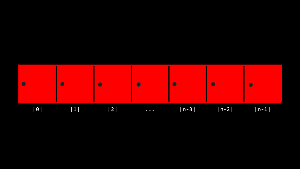
Representation for an array from CS50x

 

…The pseudocode for selection sort could be expressed like this:

 

For i from 0 to n–1
    Find smallest number between numbers[i] and numbers[n-1]
    Swap smallest number with numbers[i]

 

This animation (from here) allows us to visualize it: 

 

 

Like bubble sort, this sorting algorithm also is O(n²) (quadratic time). Its worst-case scenario would be one in which the array is in decreasing order, and has the maximum number of swaps. In terms of simplicity and ease of implementation, both algorithms are straightforward, but selection sort tends to perform better in practice due to fewer swaps.

For larger datasets, however, there are more efficient sorting algorithms. But before reviewing another algorithm, let’s talk about a very important concept: Recursion. This is a computer science concept where a function calls itself in order to solve a problem. Instead of using a loop to iterate through data, recursion relies on breaking down a problem into smaller subproblems and solving them in a recursive manner until a base case is reached.

Recursion is a powerful technique that can be used to simplify certain types of problems, but it should be used with caution to avoid infinite loops. A proper termination condition (base case) is crucial to prevent the recursion from continuing indefinitely.

For instance, let’s suppose we want a function in Python that calculates the sum of integers. The program could be like this:

 

def sum_of_integers(n):
    # Base case
    if n == 1:
        return 1
    else:
        # Recursive case
        return n + sum_of_integers(n-1)

 

In this example, the sum_of_integers function calls itself with a smaller argument, until it reaches the base case (if n == 1: return 1).

For instance, if you call sum_of_integers(5), the flow of the recursive calls for sum_of_integers(5) would look like this:

 

sum_of_integers(5) calls sum_of_integers(4)

sum_of_integers(4) calls sum_of_integers(3)

sum_of_integers(3) calls sum_of_integers(2)

sum_of_integers(2) calls sum_of_integers(1)

sum_of_integers(1) returns 1 (base case)

sum_of_integers(2) returns 2 + 1 = 3

sum_of_integers(3) returns 3 + 3 = 6

sum_of_integers(4) returns 4 + 6 = 10

sum_of_integers(5) returns 5 + 10 = 15 <-- 15 is the result.

 

As you can see, including a base case is always needed; if not present, the function would run infinitely.

Recursive solutions often provide a more concise and elegant way to express certain algorithms. They follow the "divide and conquer" paradigm, breaking down a problem into smaller subproblems and making them more organized and manageable.

We can now leverage recursion in order to explain a more efficient sorting algorithm called merge sort. It’s pseudocode would be like this:

 

MERGE SORT (array):
    If only one number
        Quit
    Else
        MERGE SORT (left half of array)
        MERGE SORT (right half of array)
        Merge sorted halves

 

Schematic example of a merge sort strategy for our example.

 

As you can see in this example, merge sort involves a recursive strategy in which the main function is called inside itself in order to divide the array into subarrays in a divide-and-conquer fashion.

Let’s suppose we’ll MERGE SORT the array [38, 27, 43, 9, 3, 82, 10]:

 

Is it one number? NO
Divide array
Left array: 38, 27, 43 | Right array: 9, 3, 82, 10
MERGE SORT(left half): 38, 27, 43
Is it one number? NO
Divide array
Left array: 38 | Right array: 27, 43
MERGE SORT(left half): 38
Is it one number? YES
MERGE SORT(right half): 27, 43
Is it one number? NO
Divide array
Left array: 27 | Right array: 43
MERGE SORT(left half): 27
Is it one number? YES
MERGE SORT(right half): 43
Is it one number? YES

 

So far we have divided the left half of the array (38, 27, 43) into its individual elements by recursively calling MERGE SORT on it. They are then rearranged in the correct order (27, 38, 43), and the same described process runs for the right half of the array (9, 3, 82, 10), which is also then rearranged (3, 9, 10, 82). Finally, both halves (now correctly ordered) are merged as a result.

Analised in terms of Big O complexity, merge sort is an example of O(n log n) (logarithm time): the first part (the “divide” part) is O(log n). Here the array is recursively divided into halves until each sub-array contains only one element. The number of divisions required is log₂n, where log₂ is the logarithm base 2. This is because, at each level of recursion, the size of the sub-arrays is halved. For example, if you have an array of 8 elements, it takes 3 divisions to reduce it to sub-arrays of size 1 (log₂8 = 3). Similarly, for an array of 16 elements, it takes 4 divisions (log₂16 = 4), and so on.

On the other hand, the second part of merge sort (the “conquer” section) would be 0(n), that is, linear time. Here, every element in the array is compared and moved once. So, the total work done in the merging step is proportional to the number of elements in the array, which is 'n'. In conclusion, the overall time complexity is the product of the logarithmic and linear parts, resulting in O(n log n).

In conclusion, in merge sort, given an input of size n, the number of steps it takes to accomplish the task are decreased by some factor with each step. That is to say that even when the number of items in an array gets bigger and bigger, the number of steps taken to order those items does not increase proportionally, but only gets “a little” bigger. This characteristic makes merge sort efficient for large datasets, especially when we can be already be sure that the items actually need ordering (because, if not, the “divide” section would be superfluous). This is because the running time of merge sort would be equally true for the worse, best and average case of merge sort: in all these cases, time complexity is the same, so it can be represented in Theta notation as ϴ (n log n).